CS 285: SOLID MODELING
Lecture #3 -- Wednesday, Sept. 7, 2011
PREVIOUS < - -
- - > CS 285 HOME < - -
- - > CURRENT < - -
- - > NEXT
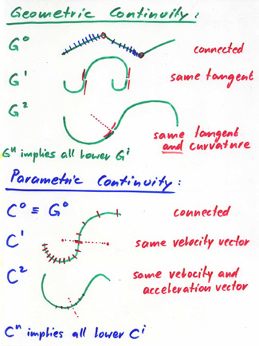
Warm-up: Geometric continuity versus Parametric continuity:
1.) Draw a curve that has G1 continuity (but not more), but does not have C1 continuity.
2.) Draw a curve that has C2 continuity, but does not have G1 continuity.
A Quick Refresher on Splines
CG Splines are linearized approximations to natural splines that minimize bending energy.
A primary concern is with the
degrees
of smoothness of these curves:
-- Parametric Continuity: differentiability of the parametric
representation (C0, C1, C2, ...)
-- Geometric Continuity: smoothness of the resulting displayed
shape (G0=C0, G1=tangent-cont., G2=curvature-cont. )
Often we distinguish
between:
-- Interpolating splines (pass through all the data points;
example Hermite splines), and
-- Approximating splines (only come close to data points; example
B-Splines).
Cubic Bezier Curves
These very handy curves are a mixture of the above two "pure" schemes.
A Cubic Bezier Curve is defined by:
-- 2 interpolated endpoints, and
-- 2 approximated intermediary control points that define the tangent
directions at the endpoints.
Cubic polynomials: ==> allow to make inflection points and true space
curves in 3D.
Basic
underlying math;
(Cubic) Polynomial: infinitely differentiable --> Continuity = C-infinity
Cubic Bezier Curve: 2 endpoints, 2 approximated intermediary control
points.
-- (P1,P2) = 1/3 of starting velocity vector
-- (P3,P4) = 1/3 of ending velocity vector
Show influence of parameters (qualitative view).
Properties of Bezier Curves
Cubic polynomial, ==> true space curves;
Infinitely differentiable; (C-infinity)
May have loops, cusps; (only G0 is guaranteed)
Interpolates endpoints;
Approximation of the two central control points;
End tangents defined by pairs of control points;
Convex hull property; (curve lies completely inside the convex hull around its control polygon)
Variation diminishing; (straight line cannot cross curve more often than control polygon)
Invariant under affine transformations; (just need to transform the control points ...)
Start-to-end symmetry; (using control points in reverse order yields the same curve)
Construction of Bezier Curves
DeCasteljau
construction algorithm: (Construction by three iterations of linear
interpolation)
Show: The role of the control points.
-- How to draw a Bezier curve from its control points:
-- Subdivision of a Bezier curve into two pieces
that together are identical to the original one.
How
to put two Bezier segments together with G1 or with C1 continuity.
This is somewhat tedious!
Cubic B-Spline Curves
An easy way to make a smooth C2-continuous space curve (for the path of an
airplane or for a moving camera)
is to sprinkle a few control points through
space that define the coarse topology and geometry of the curve
and then
let them be approximated by a
cubic B-spline.
In a nutshell, one segment depending on the 4 control points A,B,C,D,
is given by the polynomial:
Q = A(1 -3t +3t2 -t3)/6 + B(4 -6t2 +3t3)/6 + C(1
+3t +3t2 -3t3)/6 + D(t3)/6
thus the point at t=0 is given by A/6 + 4B/6 + C/6,
and the point at t=1 is given by B/6 + 4C/6 + D/6.
Assuming for the moment a closed curve with N=6 control
points,
such a curve would be described as a sequence
of N=6 cubic curve segments,
each one of which is controlled by four
consecutive control points,
(but producing a curve segment that is only
about as long as the distance between the two middle control points.)
Because
a subsequent curve segment reuses three of the control points of the previous
segment,
they blend together in a very smooth (C2-continuous) way.
Properties of Cubic B-Splines
Piecewise cubic polynomial;
Does
NOT interpolate control points;
Convex hull property;
Variation diminishing;
Construction by 3-fold linear interpolation; (similar to the one for Bezier curves)
Invariant under affine transformations;
Start-to-end symmetry;
Twice differentiable (C2) at joints;
Infinitely differentiable everywhere else;
May have cusps, thus may not even be G1, everywhere;
Good to make smooth
closed loops (and roller-coaster tracks!).
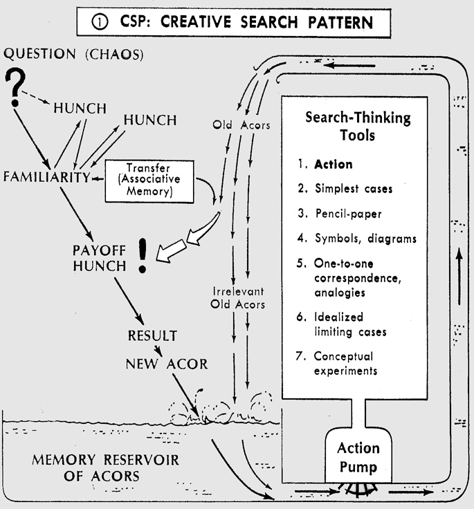
- The Creative Spark
(--> a personal mental image)
Where do you get your best ideas?
What can you do to enhance the creative flow?
Shockley's model of the "creativity pump" in the brain.
- Initial Sketch or Mock-up
(--> something that others can see)
How do you visualize, realize your ideas?
What materials may be useful to make conceptual models?
- Transformation into a CAD model
(--> something a computer can read)
How do you get those ideas into the computer?
==> Focus of your homework assignment.
- Implementation Concerns
(--> something a computer can "understand")
What do you need to do to turn that data into a solid model?
- Design Refinement
(--> something that can be physically realized)
Enter the concerns about fabrication. --> Design for manufacturing.
- Rapid Prototyping
( something that can be built on a RP machine)
What are the possibilities? Overview over various RP methods and processes (more later).
Introductions / Presentations of Assignment #1 / Discussions
Wrap-up on Space Curves and Sweeps (look at notes in Lecture #2)
The sweep parameters in SLIDE.
Procedural, Parameterized Modeling with SLIDE
Introduction to
SLIDE
-
SLIDE originated as a toy rendering system for CS 184
- SLIDE lies between Mathematica / Matlab and traditional CAD tools (Solidworks, Autocad)
- It describes boundary representations (B-reps)
- Most numerical values can be substituted by expressions that are evaluated in each rendered frame.
- It offers interactive fine tuning of critical parameters via sliders
- It builds on OpenGl (for rendering) and Tcl (user interface, expression parsing)
- Main drawbacks:
- Not a properly maintained system.
- Tcl is a pain during the debugging process!
The best way to learnSLIDE is by looking at examples, and by modifying those examples.
You should always have the SLIDE Language Specification Page open when you write SLIDE code.
Some SLIDE and Tcl Basics
Look in: http://www.cs.berkeley.edu/~sequin/CS285/CODE/
To get familiar with SLIDE, play with:
Cube.slf
BorLoopTex.slf
KG3Q60paramOptim.slf
To see what can be done with Tcl, look at:
Instancing.slf
Gear.slf
GearMovie.slf
BevelGearMovie.slf
Advice: Do not write Tcl code from scratch!
Take a working file and make very small changes between test runs.
Install SLIDE on your own computer:
A recent experience:
I found that I had to download a
different distribution than what was on
http://www.cs.berkeley.edu/~ug/slide/viewer/
Instead of
http://www.cs.berkeley.edu/~ug/slide/viewer/slide2004/slide2004.tar.gz ,
which only contained Windows-specific libraries, etc.,
I looked
http://www.cs.berkeley.edu/~ug/slide/viewer/slide2004/
and downloaded
http://www.cs.berkeley.edu/~ug/slide/viewer/slide2004/old_slide2004.tar.gz
That works fine without any need for compilation.
I just followed the
README at http://www.cs.berkeley.edu/~ug/slide/viewer/slide2004/README.
More information for the Windows system are here: http://www.cs.berkeley.edu/~ug/slide/pipeline/assignments/instructions.shtml
(see comments on "Installation")
Here is a recent report of a successful installation (by Ayden):
Copy the executable found at:
http://www.cs.berkeley.edu/~sequin/CS284/CODE/slide_subdiv.exe
Set up the following Environment Variables in Windows to run SLIDE:
(Your Computer->Properties->Advanced Settings->Environment Varibales)
ITCL_LIBRARY c:/slide/lib/itcl3.0/itcl/library
ITK_LIBRARY c:/slide/lib/itcl3.0/itk/library
Path c:\slide\bin;c:\slide\bin\SYSTEM\NT;%Path%
SLIDE_LIBRARY "c:/slide/lib"
TCL_LIBRARY c:/slide/lib/tcl8.0/library
TK_LIBRARY c:/slide/lib/tk8.0/library
Escape hatch: Later in the course you may use whatever software modeling environment you are comfortable with.
To help with creating your own environment:
Here's a link to the sweep framework (with gui) that we used in CS 184 last semester.
It should work on windows, mac and linux (tested on the hive cluster in soda 330).

http://eecs.berkeley.edu/~jima/sweep_skeletoncode_aug2011.zip
Homework Assignment (9/7 to 9/14):
PREVIOUS < - -
- - > CS 285 HOME < - -
- - > CURRENT < - -
- - > NEXT
Page Editor:
Carlo H. Séquin