To summarize, we may use divide-and-conquer to partition G0 = (N0,E0) as follows: G=(N,E) as follows:
   ( N+, N- ) = Recursive_partition( N, E )
   ... recursive partitioning routine returns N+ and N-
   ... where N = N+ U N-
       If |N| is small
           Partition G=( N, E ) directly to get N = N+ U N-
           Return ( N+, N- )
       else
(1)        Compute a coarse approximation Gc = ( Nc, Ec )
(2)        ( Nc+ , Nc- ) = Recursive_partition( Nc, Ec )
(3)        Expand ( Nc+, Nc- ) to a partition ( N+, N- )
(4)        Improve the partition ( N+, N- )
           Return ( N+, N- )
       endif
Steps (1), (3) and (4) in the above algorithm require further explanation. We describe two approaches to implementing these steps. The first approach is described in ``A fast and high quality multilevel scheme for partitioning irregular graphs'', by G. Karypis and V. Kumar; a software package implementing this method (among others) is called METIS. A similar algorithm is available in Chaco, and described in A multilevel algorithm for partitioning graphs, B. Hendrickson and R. Leland, Proc. Supercomputing '95.
The second approach is described in "A fast multilevel implementation of recursive spectral bisection for partitioning unstructured problems" by Barnard and Simon, Proceedings of the 6th SIAM Conference on Parallel Processing for Scientific Computing, 1993.
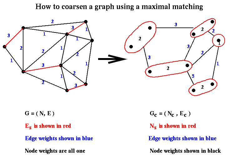
Gc is computed in step (1) of Recursive_partition as follows. We define a matching of a graph G=(N,E) as a subset Em of the edges E with the property that no two edges in Em share an endpoint. A maximal matching is one to which no more edges can be added and remain a matching. We can compute a maximal matching by a simple random algorithm:
   let Em be empty
   mark all nodes in N as unmatched
   for i = 1 to |N| ... visit the nodes in a random order
     if node i has not been matched,
        choose an edge e=(i,j) where j is also unmatched,
           and add it to Em
        mark i and j as matched
     end if
  end for
Given a matching, Gc is computed as follows. We let there be
a node r in Nc for each edge in Em. Then we
construct Ec as follows:
  for r = 1 to |Em| ... for each node in Nc
      let (i,j) be the edge in Em corresponding to node r
      for each other edge e=(i,k) in E incident on i
         let ek be the edge in Em incident on k, and
             let rk be the corresponding node in Nc
         add the edge (r,rk) to Ec
      end for
      for each other edge e=(j,k) in E incident on j
         let ek be the edge in Em incident on k, and
             let rk be the corresponding node in Nc
         add the edge (r,rk) to Ec
      end for
  end for
  if there are multiple edges between pairs of nodes of
       Nc, collapse them into single edges
Note that we can take node weights
into account by letting the weight of a node (i,j) in Nc be the sum of
the weights of the nodes i and j. We can similarly take edge weights into account
by letting the weight of an edge in Ec be the sum of the weights of
the edges "collapsed" into it. Furthermore, we can choose the edge (i,j) which
matches j to i in the construction of Nc above to have the
large weight of all edges incident on i; this will tend to minimize the weights
of the cut edges. This is called heavy edge matching in
METIS,
and is illustrated below.

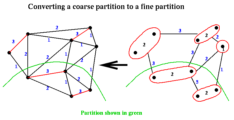
Given a partition (Nc+,Nc-) from step (2) of Recursive_partition, it is easily expanded to a partition (N+,N-) in step (3) by associating with each node in Nc+ or Nc- the nodes of N that comprise it. This is again shown below:
Finally, in step (4) of Recurive_partition, the approximate partition from step (3) is improved using a variation of Kernighan-Lin.
Now we turn to the divide-and-conquer algorithm of Barnard and Simon, which is based on spectral partitioning rather than Kernighan-Lin. The expensive part of spectral bisection is finding the eigenvector v2, which requires a possibly large number of matrix-vector multiplications with the Laplacian matrix L(G) of the graph G. The divide-and-conquer approach of Recursive_partition will dramatically decrease the cost.
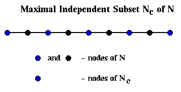
Barnard and Simon perform step (1) of Recursive_partition, computing Gc = (Nc,Ec) from G=(N,E), slightly differently than above: They find a maximal independent subset Nc of N. This means that
   Nc = empty set
   for i = 1 to |N|
      if node i is not adjacent to any node already in Nc
         add i to Nc
      end if
   end for
This is shown below in the case where G is simply a chain of 9 nodes with
nearest neighbor connections, in which case Nc consists simply of every
other node of N.
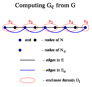
To build Ec, we proceed as follows: We will loop through the edges in E, growing "domains" Di around each node i in Nc. In other words, a domain consists of the subgraph of G connected to i by the edges examined so far. We will add an edge to Ec whenever an edge in E would connect two of these domains.
  Ec = empty set
  for all nodes i in Nc
     Di = ( { i }, empty set )  ... build initial domains
  end for
  unmark all edges in E
  repeat
     choose an unmarked edge e=(i,j) from E
     if exactly one of i and j (say i) is in some Dk
        mark e
        add j and e to Dk
     else if i and j are in different Dks (say Dki and Dkj)
        mark e
        add an edge (ki,kj) to Ec
     else if both i and j are in the same Dk
        mark e
        add it to Dk
     else
        leave e unmarked
     endif
  until no unmarked edges
For example, suppose we start with G being a chain of nodes as above, with nodes and edges numbered from left to right. Then domain Di for node i will just contain its neighbor to the right, and the edges in Ec will simply connect adjacent nodes in Nc, so Gc is just the chain of length n/2.
This completes the discussion of Barnard and Simon's implementation of step (1) of Recurive_partition.
Here is how Barnard and Simon implement step (3). Recall that the partitioning is done by using the signs of the components of the second eigenvector of the Laplacian. Assuming that we have computed an approximate second eigenvector v2 (Gc) of Gc, we must compute an approximate second eigenvector v2 (G) of G. This is done by interpolation:
  for each node i in N
     if i is also a node in Nc, then
        v2(G)(i) = v2(G1)(i),
           ... i.e. use the same eigenvector component
     else
        v2(G)(i) = average of v2(G1)(j)
           for all neighbors j of i in Nc.
     end if
  end for
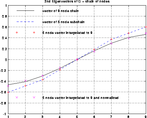
This is shown below in the case of the chain of 9 nodes. The black line
is the exact v2(G) (normalized so the sum-of-squares is one).
The dashed blue line is the exact v2(Gc), also normalized, and
which only connects every other node.
The red +'s are the approximate v2(G) computed by interpolation as
above, which by construction lie on top of the blue line.
The magenta x's are the red +'s normalized, to better see how well they
approximate the black line.
Step (4) of Recursive_partition involves refining this approximate second eigenvector to be more accurate. Refining the approximate second eigenvector can be done in several ways. (The unrefined approximate second eigenvector is not always as good as in the case of the chain!). One possibility is that the Lanczos algorithm mentioned above benefits from having a starting vector which mostly points in the direction of the desired eigenvector. More aggressively, one can use a technique called Rayleight Quotient Iteration, which uses the fact that the iteration
    choose a starting vector v(0)
            ... we use v2(Gc)
    v(0) = v(0) / norm2(v(0))
            ... norm2(x) = sqrt(sumi x(i)2)
    i=0
    repeat
       i = i+1
       rho(i) = v(i-1)' * L(G) * v(i-1)
            ... rho(i) = Rayleigh Quotient
       v(i) = ( L(G) - rho(i)*I )-1 * v(i-1)
       v(i) = v(i) / norm2(v(i))
    until convergence
converges asymptotically cubically to an eigenvalue-eigenvector pair
(rho(i),v(i)); this means the the error cubes at every step, so that for example
an error of 10-4 turns into an error of
(10-4)3 = 10-12 after one step.
rho(i) costs one matrix-vector multiply. Computing v(i), i.e.
solving the linear system (L(G) - rho(i)*I) * v(i) = v(i-1), is done using
an iterative method (called SYMMLQ) which requires yet more matrix-vector
multiplications. But since cubic convergence
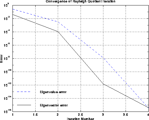
is so fast, very few steps are needed. This speedy convergence is illustrated
below by the example of the chain, where the black line is the
error in the approximate eigenvector v(i) and the dashed blue line is the
error in the approximate eigenvalue rho(i), as functions of i.
One can see the cubic convergence between iterations i=2 and i=3,
where the eigenvector error goes from 10-4 to 10-12.
Cubic convergence is only visible for this one step before hitting the
accuracy limit of 10-16 due to roundoff.
Experiments report a 10x speedup over the basic spectral bisection algorithm.
Recall that there are two classes of algorithms: geometric algorithms, that use coordinate information associated with nodes of the graph, and coordinate-free algorithm, that do not use this information. Accordingly, we present two studies comparing geometric algorithms, as well as coordinate-free ones.
We begin with geometric algorithms. The following data is taken from "Geometric Mesh Partitioning: Implementation and Experiments". Table 1 below describes the 7 graphs being partitioned. All are meshes in 2 or 3 dimensional space, rather than completely general graphs. The first four are 2-dimensional, and the last two are 3 dimensional. The fifth graph, PWT, is sometimes called "two-and-a-half dimensional", because it is a thin ("almost 2D") surface lying in 3D space. The last two columns give the number of vertices and edges in the graphs. The columns labeled "Grading" says how much larger the longest edges in the graph are than the shortest edges. For example, TRIANGLE is a regular tesselation of the place by identical equilateral triangles, so its grading is 1. AIRFOIL2 is similar to the NASA Airfoil we have seen so often, which has some large and some tiny triangles, the largest 1.3e5 times larger than the smallest.
Mesh      Description              Mesh Type
----      -----------              ---------
TAPIR     Cartoon animal           2-D acute triangles
AIRFOIL2  Three-element airfoil    2-D triangles
TRIANGLE  Equilateral triangle     2-D triangles/same size
AIRFOIL3  Four-element airfoil     2-D triangles
PWT       Pressurized wind tunnel  Thin shell in 3-space
BODY      Automobile body          3-D volumes and surfaces
WAVE      Space around airplane    3-D volumes and surfaces


Mesh      Grading   Vertices       Edges
----      -------   --------       -----
TAPIR       8.5e4       1024        2846
AIRFOIL2    1.3e5       4720       13722
TRIANGLE    1.0e0       5050       14850
AIRFOIL3    3.0e4      15606       45878
PWT         1.3e2      36519      144794
BODY        9.5e2      45087      163734
WAVE        3.9e5     156317     1059331

Table 1:  Test problems.  "Grading" is the ratio of
          longest to shortest edge lengths.
Table 2 below describes the quality of the partitioning into two subgraphs obtained by four algorithms. Quality is measured by the number of edges crossing the partition boundary, where fewer is better. The four algorithms are
Mesh     Spectral   Inertial     Default    Best
                  Partitioning   Random     Random
                                 Circle     Circle

TAPIR        59       55           37         32
AIRFOIL2    117      172          100         93
TRIANGLE    154      142          144        142
AIRFOIL3    174      230          152        148
PWT         362      562          529        499
BODY        456      953          834        768
WAVE      13706     9821        10377       9773


Table 2:  Number of edge crossings
          for two-way partitions
Finally, we use the partitioning algorithms 7 times recursively in order to partition the graphs into 2^7 = 128 separate partitions, which one would do on a 128-processor machine. Again, the quality of the partitions is largely comparable.
Mesh          Spectral        Inertial     Default
                            Partitioning   Random
                                           Circle

TAPIR           1278           1387         1239
AIRFOIL2        2826           3271         2709
TRIANGLE        2989           2907         2912
AIRFOIL3        4893           6131         4822
PWT            13495          14220        13769
BODY           12077          22497        19905
WAVE          143015         162833       145155


Table 3:  Number of edge crossings for 128-way partitions.
Now we consider coordinate-free algorithms more briefly. According to tests done by Kumar and Karypis, their implementation of multilevel Kernighan-Lin and Leland and Hendrickson's implementation provide partitions of quite similar quality, as does a hybrid multilevel method using both spectral partitioning and Kernighan-Lin. However, theirs is usually twice as fast (or more) s Leland and Hendrickson's, and many times faster than spectral partitioning.
Here is a very simple version of the physical mapping problem for DNA. A molecule of DNA is a very long string consisting of a particular sequence of amino acids chosen from a set of four, which may be called A, C, T and G. For example, one might have the sequence ACCTGACTCGAGACTCG, but many millions long. The sequencing problem is to determine this sequence for a given molecule of DNA. Current biochemical technology permits the following algorithm to be used. One can break up this long DNA string into a great many shorter fragments, which can be separated according to their amino acid sequences. The goal is to represent the original DNA as a sequence of these possibly overlapping fragments in some order. Given the sequences making up each fragment, one then knows the sequence making up the original DNA. To extract this representation in terms of fragments, the following experiments are performed. Each fragment F is allowed to bond to the DNA at a point P where the amino acid sequences match. This point is called a probe, and is typically a set of amino acids at one end of the fragment. If the probe is long enough, it will match at a unique point along the DNA. One records this information in a matrix B, which has one row for each fragment and one column for each probe, by putting a 1 at entry (F,P). One can perform the same kind of experiment to see which other fragments bond to fragment F at the same probe P, implying that they overlap. Each such bond between fragment F' and fragment F at probe P is recorded by storing a 1 at location (F',P) of the matrix B. In this way, looping through all the fragments, the matrix B is eventually filled in with ones (and zeros elsewhere), where B(F,P)=1 means that fragment F matches the DNA at probe P. This is shown below, where we have labeled the fragments in sorted order from left to right, and the probes in sorted order from left to right.
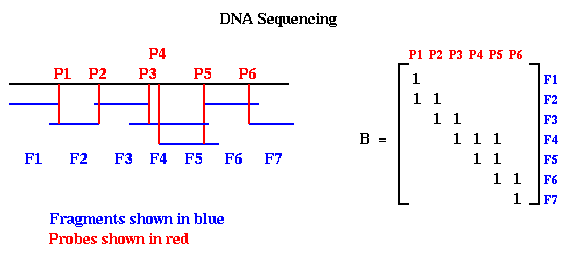
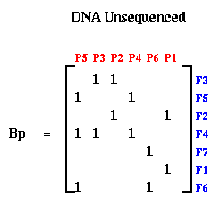
Notice that when the probes and fragments are sorted, B is a band matrix, or more precisely a consecutive-ones matrix, which means that for each row all the ones are consecutive (consecutive-ones matrices are not necessarily band matrices in the usual since, but they often are). In practice, one constructs Bp with probes and fragments in some random order, as shown below. The DNA Sequencing problem is to find the ordering of the rows and ordering of the columns of Bp which expose the underlying band matrix B, because this will say what in what order the fragments appear along the DNA.
If there were no errors in Bp, this could be done by procedure like breadth first search. But in practice, the laboratory procedure for determining entries of Bp is quite error prone, so we need a method for making Bp "close to" a band matrix in some sense. This is where spectral ordering comes in.
Let G=(N,E) be an undirected graph, and L(G) its Laplacian. Let N = N- U N+ be an arbitrary partition of the nodes, and let x be a column vector, where x(i) = +1 if i is in N+, and x(i) = -1 if i is in N-. In Lemma 1 of the last lecture, we showed that the number of edges connecting N+ and N- was equal to
.25 * sumedges e=(i,j) (x(i) - x(j))2Therefore, the partition N = N- U N+ which minimizes the number of connecting edges is given by the solution x of the minimization problem
     min[ x(i) = +1 or -1, sumi x(i) = 0 ]
             .25 * sumedges e=(i,j) (x(i) - x(j))2
The spectral partitioning algorithm involved solving the following
approximation:
     minsum_i v(i)^2 = |N|, sum_i v(i) = 0
            .25 * sumedges e=(i,j) (v(i) - v(j))2
and then choosing x(i) = sign(v(i)).
One can think of this algorithm as embedding the graph G into the real axis, putting node i at location v(i). If e=(i,j) is an edge, then we draw a line segment from v(i) to v(j), which has length |v(i) - v(j)|. The spectral bisection algorithm chooses this embedding into the real axis so as to minimize the sum of squares of the lengths of these line segments, subject to the constraints sum_i v(i)^2 = |N|, and sum_i v(i)=0.
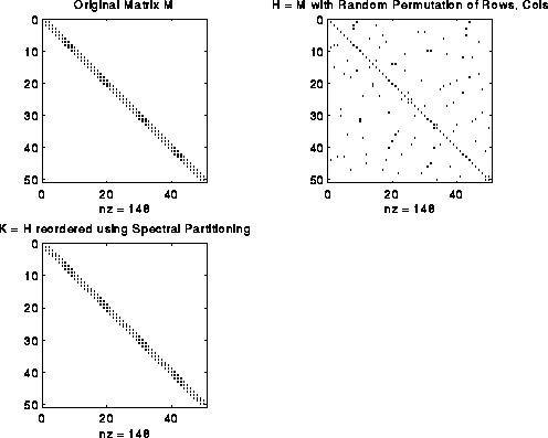
Suppose we start with a symmetric matrix H, form its graph G(H), and apply the above algorithm, yielding a second eigenvector v of L(G(H)). Let P be a permutation matrix, i.e. the identity matrix with its columns permuted, such that the entries of P*v, which are the the entries of v permuted the same way, are in sorted order. Now form K = P*H*P'. K is the matrix H with its rows and columns reordered in the same way that sorts v. The fact that the sum of all (v(i)-v(j))^2 is minimized, means that there are few edges connecting distant v(i) and v(j). In other words, if v(i) and v(j) are widely separated in the sorted list of entries of v, they are unlikely to have an edge connecting them. In the matrix K, this means that there are few nonzero entries far from the diagonal, because these would correspond to an edge from a v(i) to a v(j) widely separated in the sorted list. In other words, K is close to a band matrix.
For example, consider the matrix M = L(G), where G is a chain of n nodes. M is a tridiagonal matrix as shown in the figure below. Now perform a random permutation of the rows and columns of M to get H. H has nonzeros uniformly distributed off the diagonal. Apply spectral partitioning to H as described above to get K. As shown below, K is tridiagonal again. (The label nz under each graph is the number of nonzeros entries in the matrix.)
This bandwidth narrowing property (or, more precisely, "consecutive-one-ifying" property) is what we need to reorder the rows and columns of Bp to make it a band (or consecutive-ones) matrix. But reordering Bp requires two permutations, one for the rows and one for the columns, while spectral bisection computes just one permutation. We get around this as follows. We can write Bp = Pf*B*Pp', where Pf and Pp are two unknown permutation matrices we wish to compute; Pf shuffles the rows of B, and Pp shuffles the columns. Now consider the symmetric matrix
Tp = Bp'*Bp = (Pf*B*Pp')'*(Pf*B*Pp') = Pp*(B'*B)*Pp'
Note that Tp only depends on Pp and B, but not on Pf.
If B is a band matrix, one can confirm that B'*B is too, although with
a larger bandwidth. (If B is a consecutive-ones matrix, B'*B shares
a similar property; see
A spectral algorithm for seriation and the consecutive ones problem
for details.)
Thus, Pp can be determined just by using spectral
bisection to find the
single permutation of rows and columns of Tp that makes Pp'*Tp*Pp
(nearly) a band matrix. Similarly one can apply spectral bisection to
Tf = Bp*Bp' = (Pf*B*Pp')*(Pf*B*Pp')' = Pf*(B*B')*Pf'
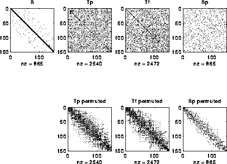
to independently determine Pf. An example is shown below, where we
start with a perfect band matrix and add a few other random entries to
get B, and randomly permute its rows and columns to get Bp.
The bottom row of three matrices shows Tp, Tf and Bp after permuting
them to make them close to band matrices.
One can see that the construction is far from "perfect", and in fact
degrades more if the random entries added to B are farther from the diagonal.
The physical mapping of DNA remains a hard problem.
The system we will describe is called PARTI, and has more recently been renamed CHAOS. This material is taken from "Distributed Memory Compiler Methods for Irregular Problems -- Data Copy Reuse and Runtime Partitioning," by J. Saltz, R. Das, R. Ponnusamy, and D. Mavripilis, ICASE Report 91-73, NASA Langley Research Center, Hampton VA, 1991.
PARTI is an extension of HPF (High Performance Fortran), and uses the features of HPF for describing array layouts across processors. We begin by reviewing data layouts.
At the end of Lecture 5, we discussed data layout in CM Fortran, where for example the declaration (KEYWORDS are capitalized)
      REAL a(64,8), b(64,8), c(64,8)
CMF$  LAYOUT a( :NEWS, :SERIAL ), b( :NEWS, :SERIAL ),
CMF$  LAYOUT c( :SERIAL, :NEWS )
indicated that A(i,j) was to be stored in the j-th memory location of processor
i, the same for B(i,j), and that C(i,j) was instead to be stored in the
i-th memory location of processor j. This would mean that the assignment
A=B could occur in parallel without communication, but that A=C would require
a great deal of communication.
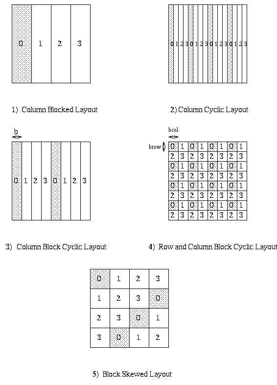
These simple layout directive are not enough for all purposes. In the beginning of Lecture 13, we discussed the more complicated data layouts required to do Gaussian elimination (or other dense linear algebra problems) efficiently on a distributed memory machine, and said the the first four of the following layouts were declarable within the HP Fortran language:
Here, very briefly, is how HPF permits users to declare these kinds of layouts. Rather than saying how each matrix entry maps to a processor location, two levels of indirection are used. The first level declaration declares how many of the available processors are to be used in the layout. A simple example is the following, which declares mygrid to be a linear array of 4 processors.
PROCESSOR mygrid(4)
The second level declares a template, or "virtual array", and
says how to lay it out on mygrid. For example
     TEMPLATE template_blocked(100),template_cyclic(100)
     DISTRIBUTE template_blocked(BLOCK) ONTO mygrid
     DISTRIBUTE template_cyclic(CYLIC) ONTO mygrid
declares that template_blocked(0:24) is mapped to processor 0,
template_blocked(25:49) is mapped to processor 1, and so on,
in general with template_blocked(i) mapping to processor floor(i/25).
Also, template_cyclic(i) is mapped to processor i mod 4.
Block cyclic layouts are also available. Multi-dimensional arrays can
have each subscript mapped independently, as preferred for Gaussian
Elimination.
A template has no memory allocated for it; it just describes a layout. The final level of declaration actually allocates memory for arrays. For example
     REAL  a(100), b(100), c(100)
     ALIGN a(i) WITH template_block(i)
     ALIGN b(i) WITH template_block(i)
     ALIGN c(i) WITH template_cyclic(i)
declares 3 arrays of 100 entries each. a(i) and b(i) are declared to
be stored at the same place as the template entry template_block(i),
in this case floor(i/25).
However template_block is DISTRIBUTEd, a(i) and b(i)
will always be on the same processor. c(i) is declared to be stored
at the same place as template_cyclic(i), that is i mod 4.
The reason for these levels of indirection is that one can independently control the amount of parallelism (via PROCESSOR), the layout (via DISTRIBUTE) and which variables are local with which other (via ALIGN).
The same mechanism can be used for more irregular layouts, but we need one more level of indirection to specify the irregularity. For example
     TEMPLATE irregular(100)
     INTEGER map(100)
     DATA map/3,2,2,1,1,1,3,0,1,2,... /
           ... 100 values from 0 to 3
     DISTRIBUTE irregular(map) ONTO mygrid
     REAL d(100)
     ALIGN d(i) WITH irregular(i)
These declarations specify that irregular(i) is mapped to processor map(i),
i.e. irregular(1) is mapped to processor map(1)=3,
irregular(2) is mapped to processor map(2) = 2, and so on.
The ALIGN statement in turn says d(1) is stored on processor 3,
d(2) is stored on processor 2, and so on.
In this example, map is specified at compile-time, and the decision about where to store d(i) is specified at compile-time. This is very limiting, since we probably won't know the actual data structure we need to partition until run-time. The extensions in PARTI to this approach are to allow map to be computed at run time (by examining some user specified loops and doing graph partitioning), and DISTRIBUTE to be executed at run-time as well, in effect recompiling the code at run-time. This is likely to be quite expensive, and so is done only when the user wants to.
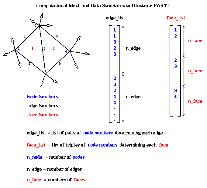
Here is an example, taken from a computational fluid dynamic (CFD) application. The data structure is a two-dimension triangular mesh, made up of nodes (numbered in blue), edges (numbered in black) and faces (numbered in red). The mesh data is stored in two arrays. The edge_list array stores a pair of nodes for each each edge: the nodes numbers for the i-th edge are stored at edge_list(i) and edge_list(i + n_edge), where n_edge is the number of edges. The face_list array stores a triple of nodes for each face: the nodes for the i-th face are stored at face_list(i), face_list(i + n_face), and face_list(i + 2*n_face), as shown below. For example, face 1 has corners at nodes 1, 2 and 3. face 2 at nodes 2, 3 and 4, and so on.
The original sequential program has two data arrays, x and y, which store data associated with each node. In other words x(i) and y(i) are data about the fluid flow at node i. The algorithm has two loops. Loop L1 below loops over all edges, and for each edge updates the data at both nodes determining that edge. Loop L2 loops over all faces, and for each face updates the data at the three nodes determining the face. The functions foo1, foo2, etc, are simple scalar functions of their scalar arguments, whose details do not concern us.
    REAL x(n_node), y(n_node)
    ...
C   Loop over all edges
L1: DO i = 1, n_edge
       n1 = edge_list(i)
       n2 = edge_list(i + n_edge)
       y(n1) = foo1(y(n1),y(n2),x(n1),x(n2))
       y(n2) = foo2(y(n1),y(n2),x(n1),x(n2))
    END DO

C   Loop over all faces
L2: DO i = 1, n_face
       n1 = face_list(i)
       n2 = face_list(i + n_face)
       n3 = face_list(i + 2*n_face)
       y(n1) = foo4(y(n1),...,x(n3))
       y(n2) = foo5(y(n1),...,x(n3))
       y(n3) = foo6(y(n1),...,x(n3))
    END DO
Here is the parallel version of this program using PARTI:
    REAL x(n_node), y(n_node)
    TEMPLATE coupling(n_node)
    DISTRIBUTE coupling(BLOCK) ONTO mygrid
    ALIGN x(i), y(i) WITH coupling(i)
    ...
C   Decide whether to redistribute data
    IF (time_to_remap) THEN
       DISTRIBUTE coupling(IMPLICIT USING L1)
    END IF
C   Loop over all edges

    IMPLICITMAP(x,y) L1
L1: DO i = 1, n_edge
       n1 = edge_list(i)
       n2 = edge_list(i + n_edge)
       y(n1) = foo1(y(n1),y(n2),x(n1),x(n2))
       y(n2) = foo2(y(n1),y(n2),x(n1),x(n2))
    END DO

C   Loop over all faces
L2: DO i = 1, n_face
       n1 = face_list(i)
       n2 = face_list(i + n_face)
       n3 = face_list(i + 2*n_face)
       y(n1) = foo4(y(n1),...,x(n3))
       y(n2) = foo5(y(n1),...,x(n3))
       y(n3) = foo6(y(n1),...,x(n3))
    END DO
Initially, the TEMPLATE coupling is laid out in a blocked fashion onto the processor grid mygrid. Arrays x and y are aligned with coupling. Later, perhaps after the arrays edge_list and face_list have been set up, the user sets time_to_remap to true, and executes the DISTRIBUTE statement following the IF statement. At this point, the system begins the "Inspection phase": It will examine loop L1, which is identified later with the IMPLICITMAP statement. The arguments x and y of IMPLICITMAP tell the system to compute the graph G of data dependencies among the references to x and y in the subsequent loop L1. This is done by executing loop L1 "symbolically", i.e. running through thg loop from i=1 to n_edge, computing the subscripts n1 = edge_list(i) and n2 = edge_list(i + n_edge), seeing that y(n1) depends on y(n1), y(n2), x(n1), and x(n2), and adding nodes n1 and n2, and edge (n1,n2), to graph G, which is initially empty. Functions foo1 and foo2 are not evaluated, and y(n1) and y(n2) are not changed. After computing G, a graph partitioning routine is called to break G into as many pieces as there are processors in mygrid. The partitioning information is stored in the TEMPLATE coupling, with coupling(i) = j if the partition algorithm puts node i onto processor j. All arrays ALIGNed with coupling (namely x and y) are redistributed according to the newly updated coupling. Finally, all parts of the program that reference arrays x or y are "recompiled" to insert the necessary communications to continue to access the data they need.
After completing the "IF (time_to_remap)" block, one reaches loop L1. At this point, the "Execute phase", the newly recompiled code is executed and array y updated. Loop L2 is executed similarly.