CS 184: COMPUTER GRAPHICS
PREVIOUS
< - - - - > CS
184 HOME < - - - - > CURRENT
< - - - - > NEXT
Lecture #28 -- Wed 5/06/2009.
Summary and Clarification:
1) What is the main characteristics of the Forward Euler method ?
2) What is the main purpose/characteristics of the Implicit Methods ?
3) How can you improve accuracy in your ODE solver ?
4) How does the Implicit Euler method gain its improved stability ?
Warm-up for AA:

|

|
A wheel with 8 spokes is turning at
a rate of 1 revolution per second.
What does the wheel appear to do
when it is rendered at 10 frames/sec.
without any anti-aliasing measures ?
(Shirley, page 495.)
|
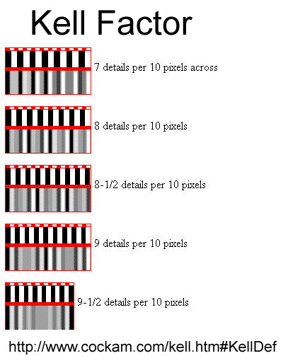
How many B&W line pairs can you draw
on a display with 1200x1200 square pixels:
(a) vertical lines in the horizontal direction ?
(b) diagonal lines between opposite corners ?Pixel Patterns Kell Factor
|
Sampling, Anti-Aliasing; Handling Texture Maps and Images
Moiré Effects
==> Demonstrate Moiré patterns with grids on VG projector.
What is going on here ? Low (spatial) frequency patterns result
from an interaction of two mis-registered grids.
What does this have to do with computer graphics ? ==> Occurs
in rendering.
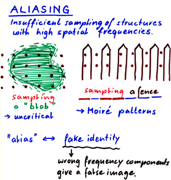
When sampling a fuzzy blob (low spatial frequencies) there is no problem, but
sampling a fence (periodic structure) at a sampling rate similar to
the lattice period will cause Moiré patterns.
Why is it called aliasing
? ==> Strong connection to signal processing!
But here we deal with a spatial/frequency domain (rather than the time/frequency domain).
To properly resolve a high-frequency signal (or spatial structure) in a sampled environment,
we must take at least TWO samples for the highest-frequency periods of the signal. This is called the Nyquist frequency limit.
Problems arise, if our signal frequency exceeds this Nyquist limit.
If our sampling frequency is too low, the corresponding humps in the frequency domain move closer together and start to overlap!
Now frequencies in the different humps start to mix and can no longer be separated (even with the most perfect filter!).
Thus some high frequency components get mis-interpreted as much lower frequencies;
-- they take on a different "personality" or become an a alias.
{The figures used here are from P. Heckbert's MS Thesis:
http://www-2.cs.cmu.edu/~ph/texfund/texfund.pdf }
What does a computer graphics person have to know ?
This occurs with all sampling techniques!
Rendering techniques that are particularly affected:
-- Ray-casting, ray-tracing: -- Because we are sampling
the scene on a pixel basis.
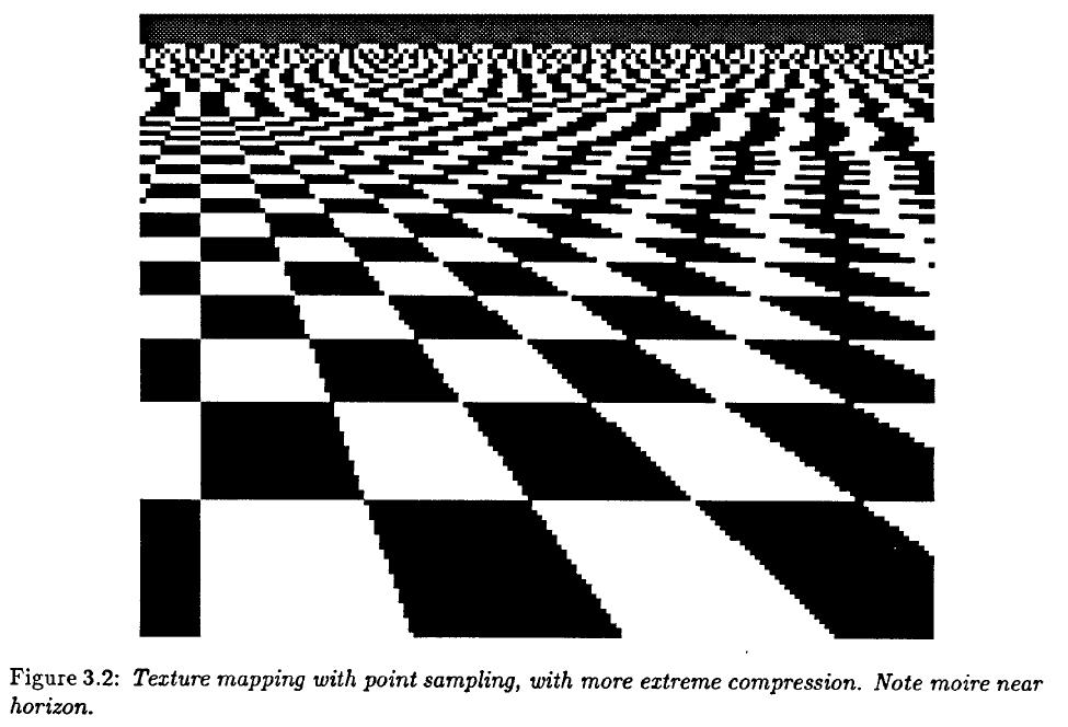
-- Texture-mapping: -- Because we use a discretely
sampled texture map.
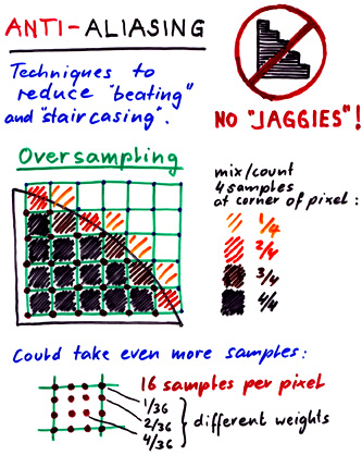
==> Fight it ! -- "NO
JAGGIES!"
-- Techniques to overcome it are
called anti-aliasing.
If we cannot increase sampling density,
then we must lower the spatial frequencies by lowpass filtering the
input -- BEFORE we sample the scene!
This cuts off the high frequency components that could cause trouble by overlapping with lower "good" frequencies.
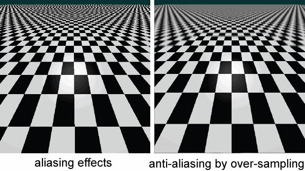
But in computer graphics we can very often get rid of aliasing by oversampling and by combining samples.
The generalization of this (multiple samples combined with different weights) is called "digital filtering."
In the context of ray-tracing we shoot multiple rays per pixel ==> Leads to "Distribution Ray Tracing".
This not only lets us gracefully filter out the higher, bothersome spatial frequencies,
it also allows us to overcome temporal aliasing problems caused by fast moving objects (e.g.. spoked wheel in warm-up question).
By taking several snapshots at different times in between subsequent frames and combining them,
we can produce "motion blur" and generate the appearance of a fast smooth motion.
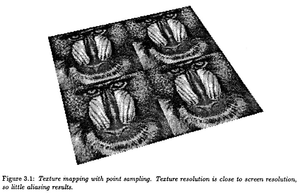
If the
frequency content of the texture pattern is close to screen resolution,
then there are no higher spatial frequencies present than what the pixel sampling can handle.
But if the texture is of much higher resolution, then there is a serious problem!
Fortunately there are filtering techniques that can fix that problem -- simple oversampling will do.
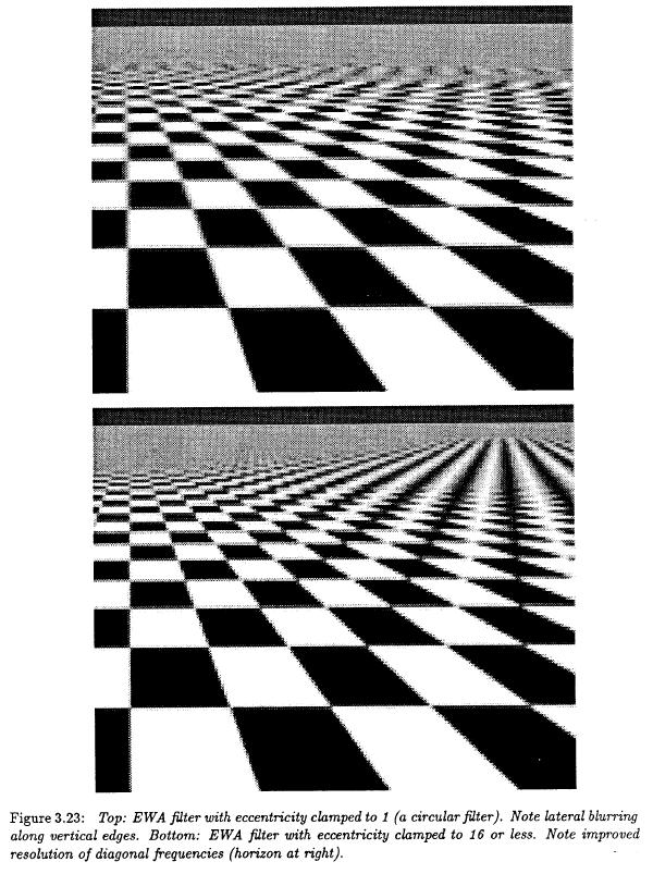
There are more advanced techniques using elliptical filtering that can give even better results.
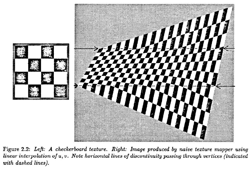
There is another issue with sampled texture patterns:
In a perspective projection, it is not good enough to determine the
texture coordinates
of the many pixels of a texture-mapped polygon simply by linear interpolation, since the
perspective projection to 2D is a non-linear operation.
If we simply linearly interpolate the texture coordinates along the edges of our polygons
(or the triangles or trapezoids that they may be cut up into), the
texture pattern will appear warped.
We need to properly foreshorten the texture coordinates with the perspective transform, so that the result will appear realistic.
There are many other applications where image sampling is crucial:
Image Stitching
Images taken from the same location, but at different camera angles need to be warped before they can be stitched together:
The original two photos at different angles. The final merged image.
To Learn More: P. Heckbert's 1989 MS Thesis: Fundamentals of Texture mapping and Image Warping.
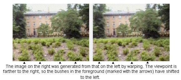
Image-based Rendering
Here, no 3D model of a scene to be rendered exists, only a set of images taken from several different locations.
For two "stereo pictures" taken from two camera locations
that are not too far apart,
correspondence is
established between key points in the two renderings (either manually, or with computer vision techniques).
By analyzing the differences of their relative positions in the two
images, one can extract 3D depth information.
Thus groups of pixels in both images can be annotated with a distance
from the camera that took them.
This basic approach can be extended to many different pictures taken from
many different camera locations.
The depth annotation establishes an implicit 3D database of the geometry
of the model object or scene.
To produce a new image from a new camera location, one selects
images taken from nearby locations
and suitably shifts or "shears" the pixel positions according to their
depth and the difference in camera locations.
The information from the various nearby images is then combined in
a weighted manner,
where closer camera positions, or the cameras that see the surface of interest under a
steeper angle, are given more weight.
With additional clever processing, information missing in one image
(e.g., because it is hidden behind a telephone pole)
can be obtained from another image taken from a different angle,
or can even be procedurally generated by extending nearby texture patterns.
Example 1: Stereo
from a single source:
A depth-annotated image of a 3D object, rendered from two different
camera positions.
Example 2: Interpolating an
image from neighboring positions:
To Learn More: UNC Image-Based Rendering
Future Graduate Courses: 283, 294x ...
Light Field Rendering
These methods use another way to store the information acquired from a
visual capture of an object.
If one knew the complete 4D plenoptic function (all the photons
traveling in all directions at all points in space surrounding an object),
i.e., the visual information that is emitted from the object in all
directions into the space surrounding it,
then one could reconstruct perfectly any arbitrary view of this object
from any view point in this space.
As an approximation, one captures many renderings from many locations
(often lying on a regular array of positions and directions),
ideally, all around the given model object, but sometimes just from
one dominant side.
This information is then captured in a 4D sampled function (2D
array of locations, with 2D sub arrays of directions).
One practical solution is to organize and index this information (about
all possible light rays in all possible directions)
by defining the rays by their intercept coordinates (s,t) and (u,v)
of two points lying on two parallel planes.
The technique is applicable to both synthetic and real worlds, i.e.
objects they may be rendered or scanned.
Creating a light field from a set of images corresponds to inserting
2D slices into the 4D light field representation.
Once a light field has been created, new views may be constructed by
extracting 2D slices in appropriate directions.
"Light Field Rendering":
Example: Image
shows (at left) how a 4D light field can be parameterized by the
intersection of lines with two planes in space.
At center is a portion of the array of images that constitute the entire
light field. A single image is extracted and shown at right.
Source: http://graphics.stanford.edu/projects/lightfield/
To Learn More: Light
Field Rendering by Marc Levoy and Pat Hanrahan
Future Graduate Courses: 283, 294x ...
HKN Survey
Read Chapter 25 in Shirley; Skim Sections 4.4 and 4.5 in Shirley.
Study whatever gives you the needed background information for your project.
Second intermediate report (="AS#10"), Due: FRIDAY, May 8, 2009.
Explain briefly (1 - 5 sentences) what you have constructed so far for your project,
and upload an image of a relevant piece of geometry created for your project.
PREVIOUS
< - - - - > CS
184 HOME < - - - - > CURRENT
< - - - - > NEXT
Page Editor: Carlo
H. Séquin