Back Face Culling Notes

• Back Face Culling
• Transforming Planes
• Transforming Normals
• Computing the Best Fit Plane for a Polygon Loop

Back Face Culling

Back face culling is when you do not render a polygon because its normal is pointing away from the viewer's eye point. A naive way of preforming this check would be to construct a vector from the eye point to a point on the face and compute the dot product of this line of sight vector and the normal vector. If this scalar is positive then the face is pointing away and consequently can be culled. A more sophisticated way of making this check is to transform the face's normal into the projection space, where the line of sight vector is always the negative Z-axis. Then the check for back face culling is just to see if the Z component of the transformed normal is negative.

The problem now is to find a way to transform face normals, and to find a good representation for the normal to make this transformation easy.

Transforming Planes

If we have a plane vector n = [a, b, c, d] which describes a plane then for any point p = [x, y, z, 1] in that plane the follow equation holds:

n^t p = ax + by + cz + d = 0

If for a point p on the plane, we apply an invertible transformation R to get the transformed point p₁, then the plane vector n₁ of the transformed plane is given by applying a corresponding transformation Q to the original plane vector n where Q is unknown.

p₁ = R p
n₁ = Q n

n₁^t p₁ = 0

(Q n)^t (R p) = 0
n^t Q^t R p = 0

Q^t R = I
Q^t = R^-1
Q = (R^-1)^t

n₁ = Q n = (R^-1)^t n

Transforming Normals

Transforming normals is very similar to transforming planes. A normal norm can be represented by a vector norm = [a, b, c, 0]. This is equivalent to the plane perpendicular the normal and passing through the origin n = [a, b, c, 0]. If we then transform this plane vector by (R^-1)^t, we will correctly transform the normal for a certain set of transformations:

This set of transformations includes our ordinary modelling transformations and the parallel projection transformation where our transformation matrices are always of the form:

For this set of transformations, the d component of n has no effect on the transformed normal direction norm₁ because it is multiplied by 0 in the terms for the a₁, b₁, and c₁ components. But our transformations will not stay in this family once we introduce the perspective projection transformation, so we might as well compute and use the full plane equations for our face normals.

So we will represent the normal of face by the best fit plane vector for that face n = [a, b, c, d] where for a point p = [x, y, z, 1] on the face the follow equation holds:

Now when we apply (R^-1) to n:

we will correctly transform the plane and consequently the normal. We are only interested in the orientation of this plane equation, so we can forget the d₁ component of n₁ to get norm₁ = [a₁, b₁, c₁]. norm₁ can then be normalized to unit length if necessary.

This is very close to being correct, but unfortunately plane equations have one less degree of freedom than normal vectors. So after the plane vector is transformed the [a₁, b₁, c₁] components can equal either norm₁ or -norm₁. Fortunately, we can distinguish between these two cases by looking at the determinant of the transformation matrix R.

Det(R) switches sign for every scale transformation with an odd number of negative scale components.

Computing the Best Fit Plane for a Polygon Loop

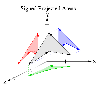
We will use Newell's algorithm for computing the normal for a polygon loop which may have noisy data. This algorithm comes close to making a least squares best fit, but computes it in a closed form. This algorithm makes use of the fact that the components of the normal of a polygon are proportional to the signed projected areas of the polygon onto the YZ, XZ, and YZ planes. In the figure below, the white polygon's normal norm = [Area(Proj_YZ), Area(Proj_XZ), Area(Proj_XY)].

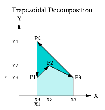
The areas of the projected polygons can be computed by treating each edge of the projected polygon as a trapezoid with a signed area. In the example below we are looking at the projection onto the XY plane, so the area is proportional to the Z component of the normal. The formula for the area of the trapezoids shown is

The areas of the trazepoids who are constructed from left pointing polygon edges are considered positive, right pointing polygon edges are considered negative, and vertical edges make zero areas. This follows from the area formula. This choice of sign is consistent with our standard counterclockwise polygon loop orientation. In the figure below, positive trapezoids ([P₃, P₄]) are colored blue, negative trapezoids ([P₁, P₂] and [P₂, P₃]) are colored white, and zero trapezoids ([P₄, P₁]) do not appear. The net area appears in blue and the areas where positive and negative trapezoids cancel appear in lighter blue.

Formula

With this in mind, if we are given a polygon described by a list of vertices p₁, p₂, p₃, ... p_n. We can find a normal vector norm = (n_x, n_y, n_z) whose components are equal to the signed projected areas of the polygon using these equations:

where x_n+1 = x₁, y_n+1 = y₁, and z_n+1 = z₁.

Then we need to find the d value for the complete plane equation n = [a, b, c, d]. We pin down the specific plane by using a p_mean which is the average of the vertex values for x, y, and z. We can then find d using norm and p_mean:

Now n = [norm, d] = [a, b, c, d] which is the plane equation that best fits the list of vertices of the polygon contour.

References

• Computer Graphics: Principles and Practice, Foley, vanDam, Feiner, and Hughes, pp. 663-664}
• Computer Graphics: Principles and Practice, Foley, vanDam, Feiner, and Hughes, pp. 216-217}
• Computer Graphics: Principles and Practice, Foley, vanDam, Feiner, and Hughes, pp. 476-477}